Introduction to tidy spatial networks
Written and presented by Stéphane Guillou Technology Trainer, UQ Library Mastodon: @stragu@mastodon.indie.host
This tutorial is an introduction to dealing with tidy spatial networks in R, demonstrating a full process of data acquisition from the open spatial database OpenStreetMap, data preparation, and basic network analysis like isodistance and shortest path calculation. Along the way, we use the default plotting methods for spatial network objects, but also make use of the ggplot2 and tmap packages as alternatives.
Setting up
To follow this tutorial, you will have to have a number of packages available, which can be best sorted out with the following command:
install.packages(c("dplyr", "ggplot2", "sfnetworks", "tmap", "osmdata"))If you run into issues installing and running sf (which relies on spatial libraries external to R), please refer to their installation instructions.
sfnetworks
The main package this tutorial centres around is the sfnetworks package (Lucas van der Meer, Lorena Abad et al.), which is the result of joining what the tidygraph package does for networks with what the sf package does for spatial vector data.
The data structure central to this package is a combination of two spatial objects, one describing the nodes (or points) and another describing the edges (or lines connecting the points). In the words of the developers:
“A close approximation of tidyness for relational geospatial data is two sf objects, one describing the node data and one describing the edge data.”
In other words, an sfnetwork object is made up of one sf object for nodes and one sf object for edges. (As opposed to two simple data.frames for a tidygraph object.)
A visual explanation of sf objects by Allison Horst (copyright hers): a dataframe with sticky geometries in a list column. The geometries are “sticky” because they don’t vanish when, say, you select() columns.
In the edges component of a network, it is also possible (or necessary) to specify where the edge starts and finishes, using the from and to columns. Such information can be interpreted as the direction of the edge in a “directed” network, or simply as its two extremities in the case of an “undirected” network.
Finally, another important characteristic of the edges is their weight. This can relate to any kind of information, but if we are interested in distances between points, it will typically be the length of the edges.
From OSM data to an sfnetwork
Although the structure of an sfnetwork seems to be quite complex, it is possible – and useful! – to use a shortcut and create one from a simple collection of linestrings.
We can download download data from a spatial vector database like OpenStreetMap (OSM), focus on the lines (or “ways”) and convert that sf object into an sfnetwork that will use the lines as edges, and their endpoints as nodes.
Let’s first download from OSM all the ways that are primary used by pedestrians in the suburb of West End. (To understand how these features are tagged in the database, a good starting point is the Map Features page on the OSM wiki.)
library(osmdata)# build the query
we_foot <- opq("west end, meanjin") %>%
add_osm_features(features = c('"highway"="footway"',
'"highway"="steps"',
'"foot"="yes"',
'"highway"="living_street"')) %>%
osmdata_sf()The osmdata package allows building Overpass queries to download OSM vector data that matches our criteria:
- Features tagged as
highway=footway, including footpaths, crossings… - Features tagged as
highway=steps, for stairs - Features tagged as
foot=yes, for example bikeways on which foot traffic is allowed (see this shared bikeway for an example) - Features tagged as
highway=living_street, a shared road on which pedestrians often have right of way
Finding the right combination of OSM tags to use is always an iterative process, refining the selection at each step.
We choose to return an sf object, which might contain points, lines and polygons. We are only interested in the lines:
names(we_foot)## [1] "bbox" "overpass_call" "meta"
## [4] "osm_points" "osm_lines" "osm_polygons"
## [7] "osm_multilines" "osm_multipolygons"we_foot_lines <- we_foot$osm_linesWe can visualise the resulting object with the sf package:
library(sf)
we_foot_lines %>%
  st_geometry() %>%
  plot()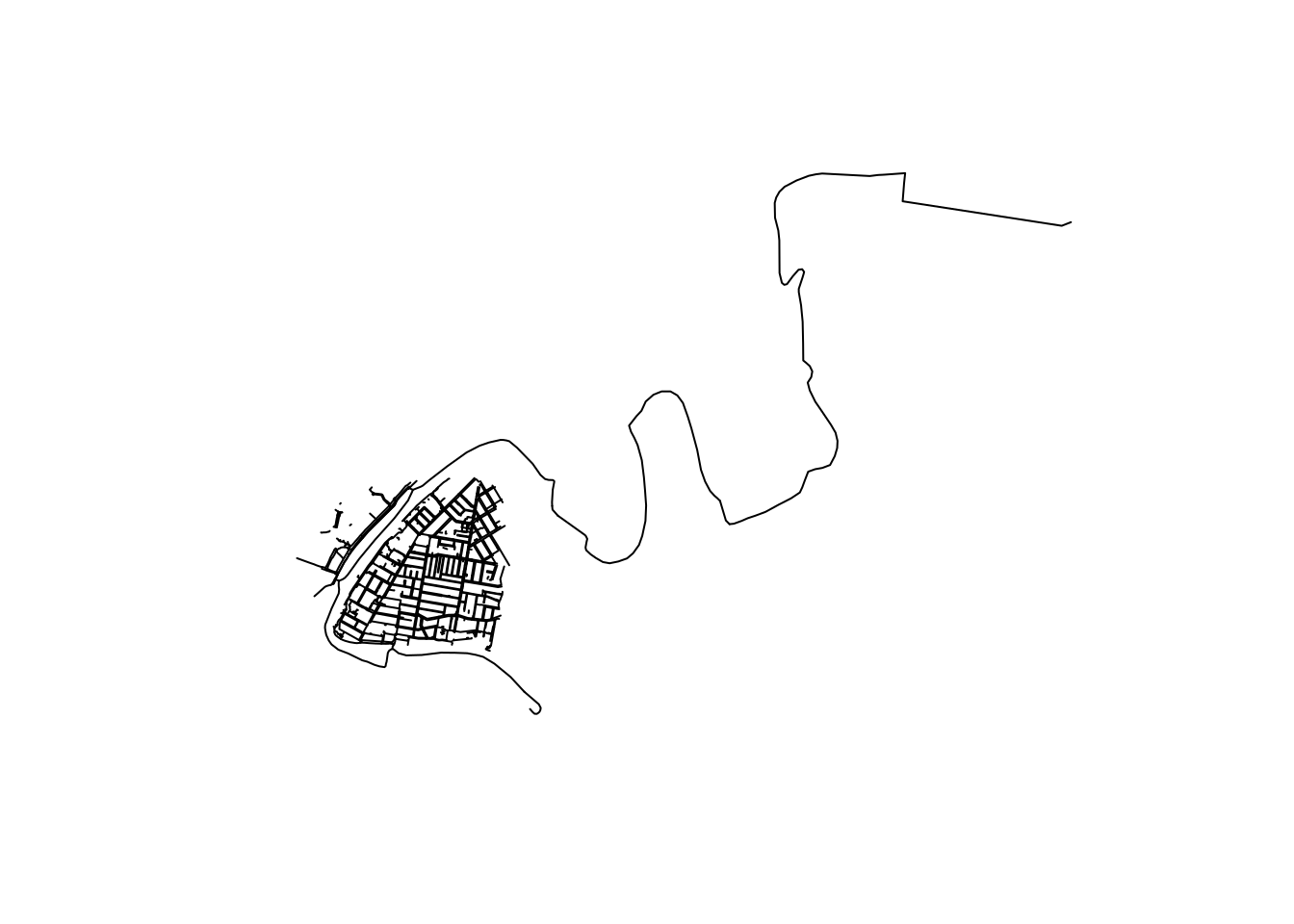
It seems to have kept a ferry route, which was tagged with foot=yes and route=ferry on OSM. We can remove it:
library(dplyr)
we_foot_lines <- we_foot_lines %>%
  filter(is.na(route))
Another caveat in our process is that some footpaths are mapped as closed ways on OSM, and are therefore returned as a polygon:
we_foot$osm_polygons %>%
  st_geometry() %>%
  plot()
The smaller ones are proper pedestrian areas, but the bigger ones are probably footpaths encircling a whole residential block. It is possible to “cast” these polygons as ways and include them in the network:
# cast polygons to lines
poly_to_lines <- st_cast(we_foot$osm_polygons, "LINESTRING")
# bind all lines together
library(dplyr)
we_foot_lines <- bind_rows(we_foot_lines, poly_to_lines)
This is what we are left with:
# plot it
we_foot_lines %>%
  st_geometry() %>%
  plot()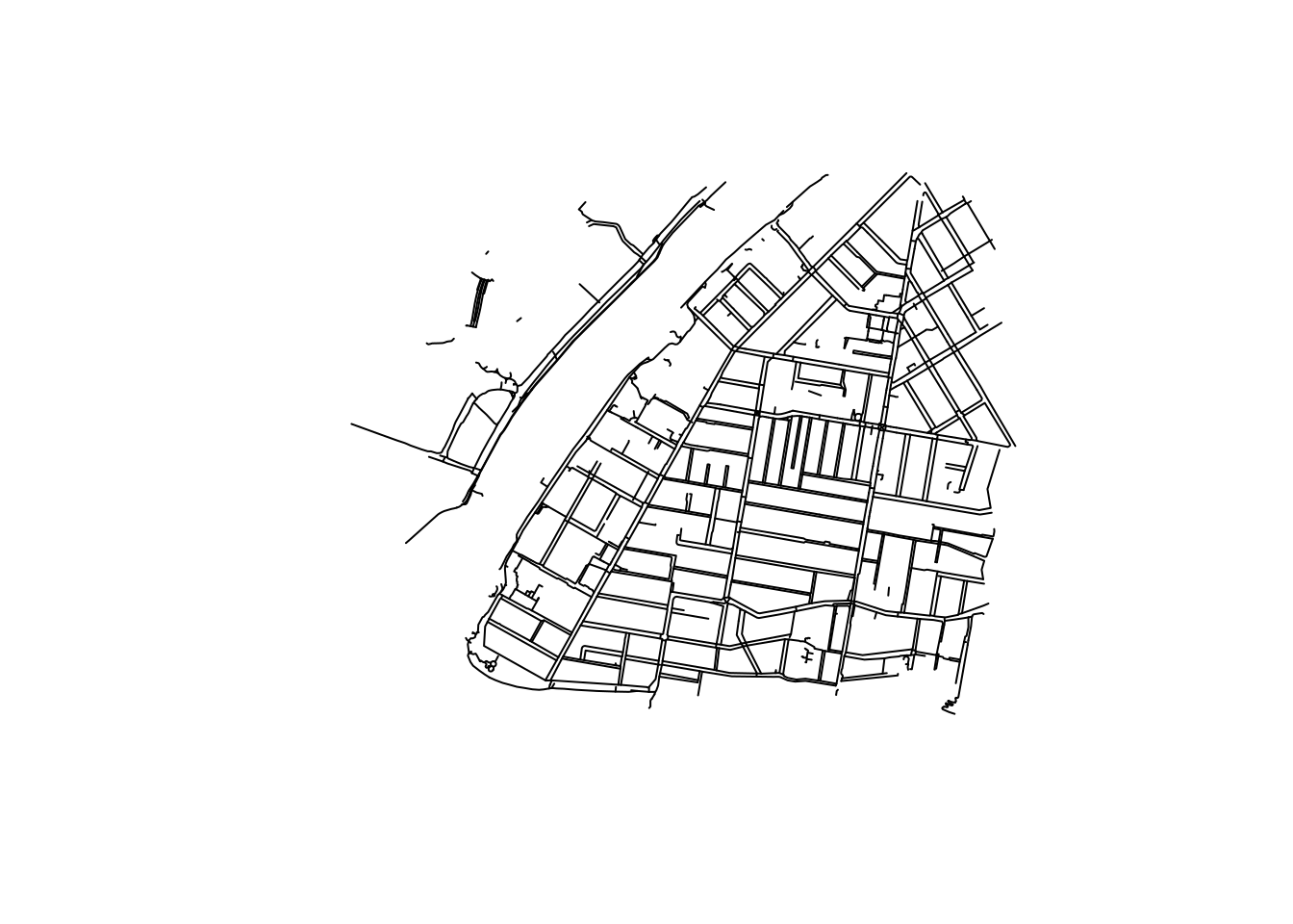
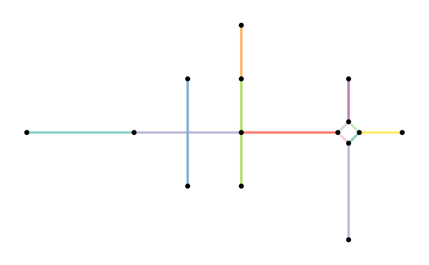
We can now convert the object to an sfnetwork object, making sure we set it as undirected (the default is directed = TRUE):
library(sfnetworks)
foot_net <- as_sfnetwork(we_foot_lines, directed = FALSE)
plot(foot_net)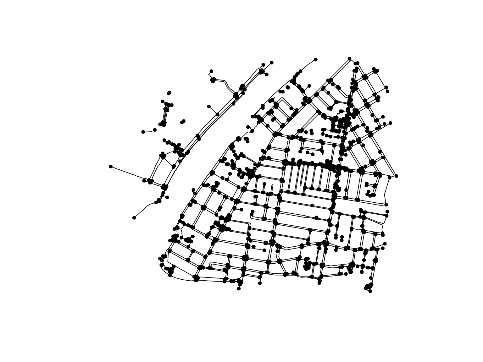
Prepare the network
CRS
The current coordinate system for the network is a global one, EPSG:4326.
st_crs(foot_net)## Coordinate Reference System:
## User input: EPSG:4326
## wkt:
## GEOGCRS["WGS 84",
## ENSEMBLE["World Geodetic System 1984 ensemble",
## MEMBER["World Geodetic System 1984 (Transit)"],
## MEMBER["World Geodetic System 1984 (G730)"],
## MEMBER["World Geodetic System 1984 (G873)"],
## MEMBER["World Geodetic System 1984 (G1150)"],
## MEMBER["World Geodetic System 1984 (G1674)"],
## MEMBER["World Geodetic System 1984 (G1762)"],
## ELLIPSOID["WGS 84",6378137,298.257223563,
## LENGTHUNIT["metre",1]],
## ENSEMBLEACCURACY[2.0]],
## PRIMEM["Greenwich",0,
## ANGLEUNIT["degree",0.0174532925199433]],
## CS[ellipsoidal,2],
## AXIS["geodetic latitude (Lat)",north,
## ORDER[1],
## ANGLEUNIT["degree",0.0174532925199433]],
## AXIS["geodetic longitude (Lon)",east,
## ORDER[2],
## ANGLEUNIT["degree",0.0174532925199433]],
## USAGE[
## SCOPE["Horizontal component of 3D system."],
## AREA["World."],
## BBOX[-90,-180,90,180]],
## ID["EPSG",4326]]st_transform() allows us to transform the coordinates to a different projection. For this part of the world, a recent Projected Reference System is EPSG:7856 (or “GDA2020 / MGA zone 56”).
foot_net <- st_transform(foot_net, 7856)If the command above gives you a GDAL error, reassign the original CRS first: st_crs(foot_net) <- 4326
Clean up
sfnetworks and tidygraph include many pre-processing and cleaning functions for graphs, some of them detailed in this article.
One relevant example for this dataset is the subdivision of edges: because some edges have interior nodes that are endpoints of other edges, they will not be connected to each other when analysing the network.
 We need to combine tidygraph’s
 convert() function with a “spatial morpher” function from sfnetworks:
library(tidygraph)
foot_net <- convert(foot_net, to_spatial_subdivision)
The network should now contain more edges.
Note that this will only happen for features sharing a node: if two edges overlap, like for bridges and underpaths, no extra node will be created where they cross, and therefore no new connecting endpoints will be created for them – which is good news!
Also note that using to_spatial_subdivision() will copy tags into each of the subdivisions of an edge. This usually isn’t a problem (think speed limits, surface, lighting, width…) but can be in some cases (for example if the length of the edge had already been added). The order of processing often matters.
Another example is the removal of nodes that have only two edges connected, also called “smoothing of pseudo-nodes”. This would be useful to simplify a network and reduce the processing times needed. We again use a combination of convert() with the relevant spatial morpher, to_spatial_smooth():
foot_simple <- convert(foot_net, to_spatial_smooth)
plot(foot_simple)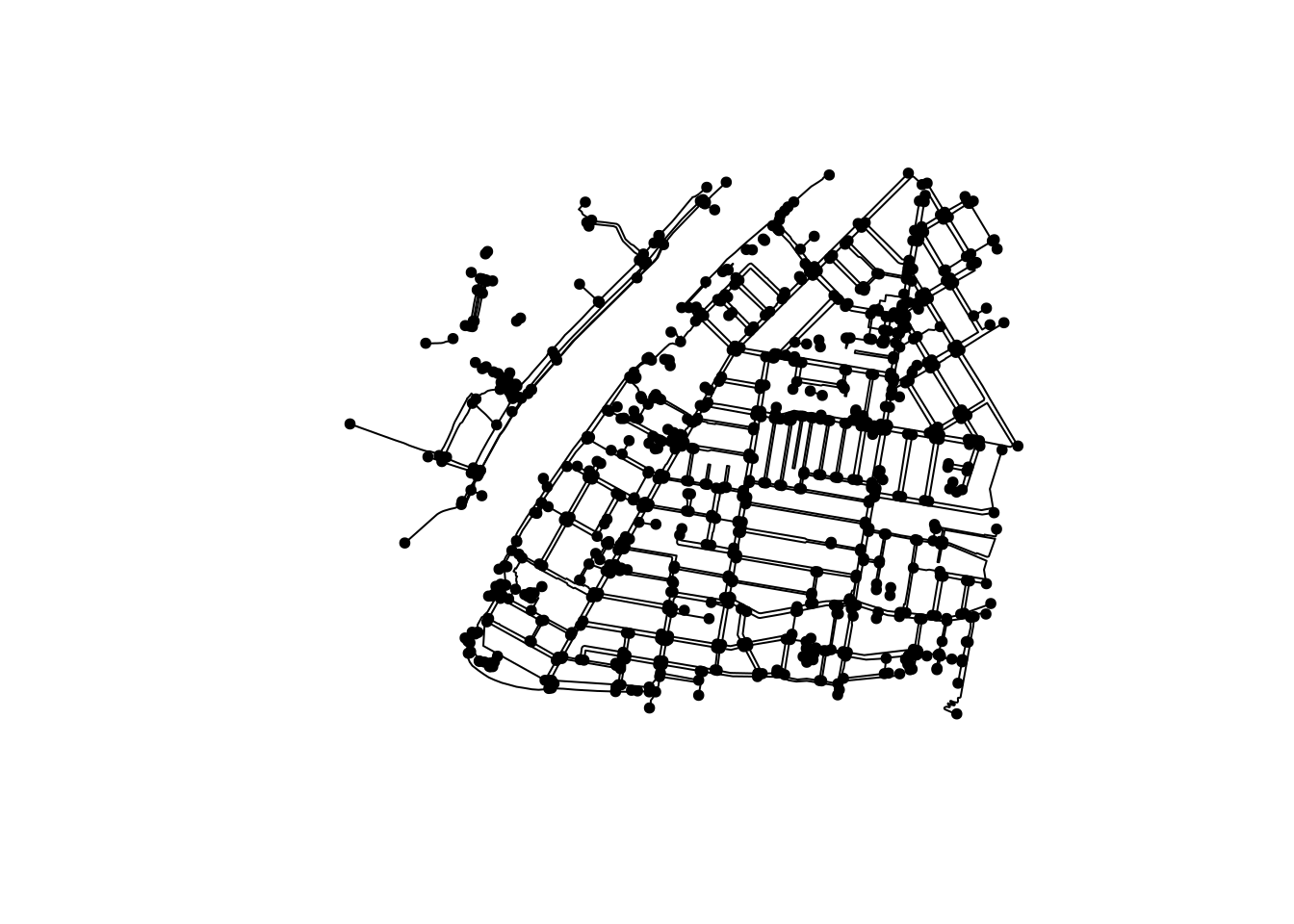
For our example, simplifying the network might not be useful:
- If we calculate isodistances or isochrones, reducing the number of nodes will reduce the precision;
- Once again, one needs to take care of the potential loss of valuable data. For example, do nodes contain relevant tags, like ones describing physical barriers? And how will the combined edges’ tags be stored?
More information about “spatial morphers”, including what options exist for dealing with attributes when multiple features are merged, is available in the documentation: ?spatial_morphers
Weights
As mentioned before, a common weight associated with each edge of the network is the edge’s length. We can add this weight to our network, but we need to first “activate” the part of the object we want to modify:
foot_net <- foot_net %>%
  activate("edges") %>%
  mutate(weight = edge_length())
Using st_as_sf(), we can extract the components of an sfnetwork object and use them in a familiar plotting system like ggplot2:
library(ggplot2)
ggplot() +
  geom_sf(data = st_as_sf(foot_net, "edges"),
          mapping = aes(colour = as.numeric(weight))) +
  labs(colour = "Edge length (m)")
Interactive map
At this point, it might be interesting to create an interactive visualisation to zoom into, which might help spot issues with the data.
library(tmap)
tmap_mode("view") # set to interactive mode
tm_tiles("CartoDB.Positron") +
tm_shape(st_as_sf(foot_net, "edges")) +
  tm_lines(col = "footway", palette = "Accent", colorNA = "red") +
tm_shape(st_as_sf(foot_net, "nodes")) +
  tm_dots()
Remove small disconnected neighbourhoods
There are a few “islands” in the network, in which not many points are connected to each other. We can remove those, by:
- Choosing how far we look to determine the size of a neighbourhood, with tidygraph’s
local_size()function - Only keeping the neighbourhoods that have reached that threshold.
foot_net <- foot_net %>%
  activate(nodes) %>%
  mutate(neighbourhood = local_size(order = 6)) %>%
  filter(neighbourhood > 5)
Isodistances
Let’s now draw an isodistance around the Kurilpa Library in West End. First, download the library’s feature from OSM, and calculate its centroid (because it is mapped as a building):
kurilpa_lib <- opq_osm_id(id = 523925261, type = "way") %>%
  osmdata_sf() %>%
  .$osm_polygons %>%
  st_centroid() %>%
  st_set_crs(4326) %>% # (if the following step generate GDAL error)
  st_transform(crs = 7856)
Then, calculate the isodistance for a distance smaller or equal to 1 km (more or less a 15-minute walk), using the node_distance_from() function from tidygraph:
foot_net <- activate(foot_net, "nodes")
iso <- foot_net %>%
  dplyr::filter(node_distance_from(st_nearest_feature(kurilpa_lib, foot_net), weights = as.numeric(weight)) <= 1000)
Finally, draw a polygon around the isodistance, and plot everything:
iso_poly <- iso %>%
  st_geometry() %>%
  st_combine() %>%
  st_convex_hull()
plot(foot_net, col = "grey")
plot(iso_poly, col = NA, border = "black", lwd = 3, add = TRUE)
plot(iso, col = "lightgreen", add = TRUE)
plot(kurilpa_lib, col = "red", pch = 8, cex = 2, lwd = 2, add = TRUE)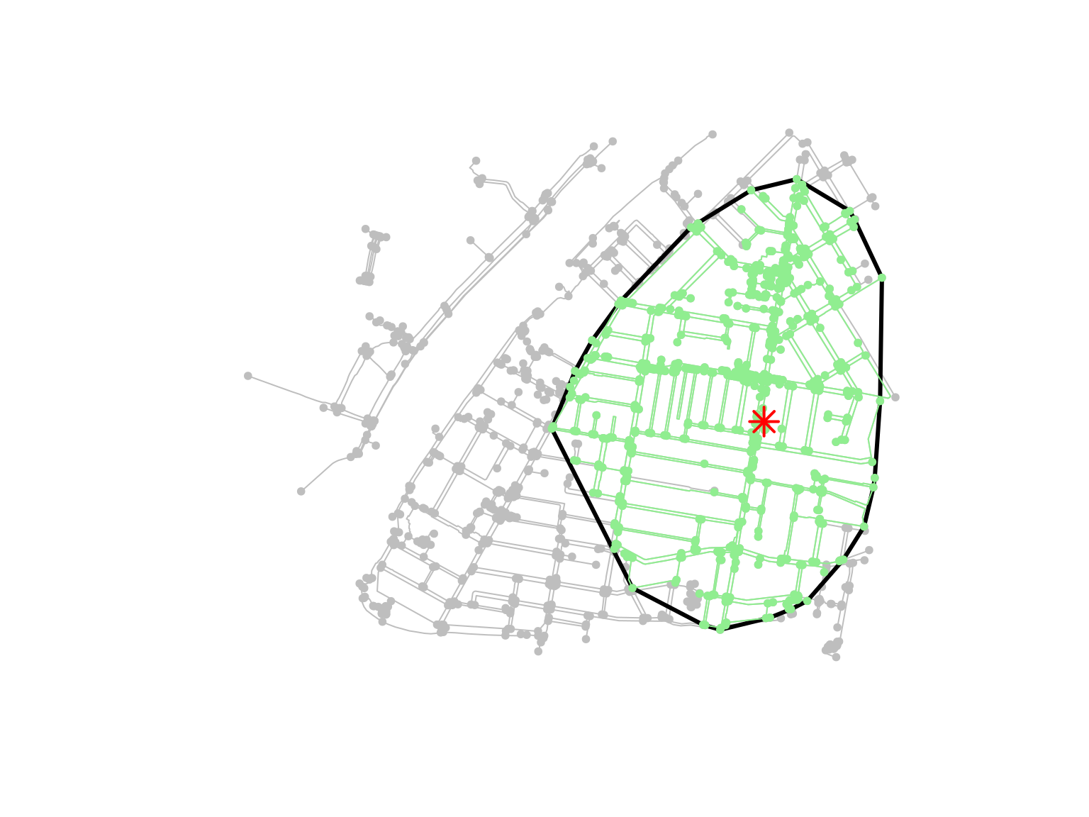
Shortest path
Let’s now calculate the shortest distance from the South Brisbane Sailing Club to the library.
# get the location of the Sailing Club's entrance
sailing_club <- opq_osm_id(id = 7622867925, type = "node") %>%
  osmdata_sf() %>%
  .$osm_points %>%
  st_set_crs(4326) %>% # (if the following step generates a GDAL error)
  st_transform(crs = 7856)

# calculate the shortest path
shortest <- foot_net %>%
  activate(edges) %>%
  st_network_paths(from = sailing_club, to = kurilpa_lib)

# extract the node IDs
node_path <- shortest %>%
  slice(1) %>%
  pull(node_paths) %>%
  unlist()

# only keep the network for these nodeIDs
path_sf <- foot_net %>%
  activate(nodes) %>%
  slice(node_path) %>%
  st_as_sf("edges")

# visualise
tm_tiles("CartoDB.Positron") +
tm_shape(path_sf) +
  tm_lines(col = "red") +
tm_shape(sailing_club) +
  tm_dots(col = "blue", size = 0.1) +
tm_shape(kurilpa_lib) +
  tm_dots(col = "green", size = 0.1)
The granularity of the OSM data available for this area allows us to create a precise path for pedestrians, switching sides of roads only when a crossing is reached. However, every new analysis of the network might reveal more interesting information about the data we have used. For example, the shortest path calculated might go through private residential paths (usually blocked by gates), and avoiding those would mean extra steps in pre-processing (for example keeping track of existing OSM tags like barrier=* on nodes and access=private on ways).
Further resources
- sfnetworks’ documentation, including its 5 articles, which inspired much of this tutorial
- tidygraph’s gigantic collection of graph manipulation functions
- Transportation chapter in the free Geocomputation with R book (Lovelace, Nowosad, Muenchow)
- Spatial network analysis with the {sfnetworks} package, video on analysing OSM data with sfnetworks, by Renate Thiede, for R-Ladies Johannesburg (2021)
- Spatial networks in R with sf and tidygraph, article by van der Meer, Abad and Lovelace (2019)
- Other related packages:
ggraph for graph visualisation
stplanr for sustainable transport planning and modeling
cppRouting for calculating distances, shortest paths and isochrones/isodistances
dodgr for distance and time calculations on directed graphs (and its vignette on street network routing based on OSM data)
osrm for using a routing API based on OSM data
Legal
Apart for illustrations in which the copyright is mentioned, this article is released under a CC-BY 4.0 licence. All data used for the data visualisations use OpenStreetMap data, which is © OpenStreetMap contributors but released under an ODBL licence.
Updates
This article was updated after it was presented:
- 2022-04-27:
- Clarify information about overlapping ways being left alone by
to_spatial_subdivision() - Add Renate Thiede’s excellent video on the exact same topic, discovered after finishing writing
- Add author’s role and contact
- Clarify information about overlapping ways being left alone by
About the Author

Stéphane is a software trainer at the UQ Library, specialising in open research software and data analysis support. After a few years working in plant science and agricultural research, he joined the great Library team where he is able to promote Open Research practices to the wider UQ community.