Creating a geospatial blog with blogdown
In this post, we will go through the process of creating a geospatial blog, specifically this blog.
First, we will run through how to create a site and host it through github and netlify. Then we will show you the options for publishing both a raster and vector data.
Part 1. Create a site and host it on Github and Netlify
Good resources
Prerequisites
- Fairly recent version of R studio (RStudio IDE version, v1.4.1106 +)
- Github account
- GIT locally on computer. (Happy git with R https://happygitwithr.com/)
- gitforwindows.org
- Download GNU
- Default on all settings Make sure to select Git from the command line and also from 3rd party software
- Sign up for Netlify using Github account
1. Create a new github repository
Initialise with readme, but don’t add the .gitignore file. Then copy link https link.
2. Create a new project in R studio
In R studio, go to File > new project > Version control > git, and Paste the URL from before. Save the project somewhere sensible.
Now install blogdown with Install.packages(“blogdown”), and load with library(blogdown).
install.packages("blogdown")
library(blogdown)Now to create a new site, just add
new_site()This will give the default theme, but there are a lot of different themes to choose from!
Its important to find one that you like, but also that is up to date and works. For this blog, we ended up going with https://themes.gohugo.io/themes/anatole/ over some other options which were buggy, probably due to being out of date.
So to build the site with your theme of choice, run
new_site(theme = "lxndrblz/anatole")Adding theme= “gighubusername/themerepo” of the theme you choose.
When prompted, select y to let blogdown start a server. This will let you preview the site in the viewer. To view in a browser, click the show in new window (next to the broom) to launch it locally.
Generally, you can serve the site, and stop serving the sites using
blogdown::serve_site() #to serve the site locally
blogdown::stop_server() #to stop serving the site3. Write a post
Hopefully the local site is working. We can now add a new blog post using either
blogdown::new_post() OR, a better method is to navigate through addins dropdown (under help, right of git icon), click new_post. This brings up a dialog to fill out.
Select file type, markdown for simple text, or .Rmd or .Rmarkdown for embedding code.
Now we can add code chunks! The easiest way to do this is to click the green +c just above the editor.
As an example
library(ggplot2)
ggplot(Orange, aes(x = age,
y = circumference,
color = Tree)) +
geom_point() +
theme_bw()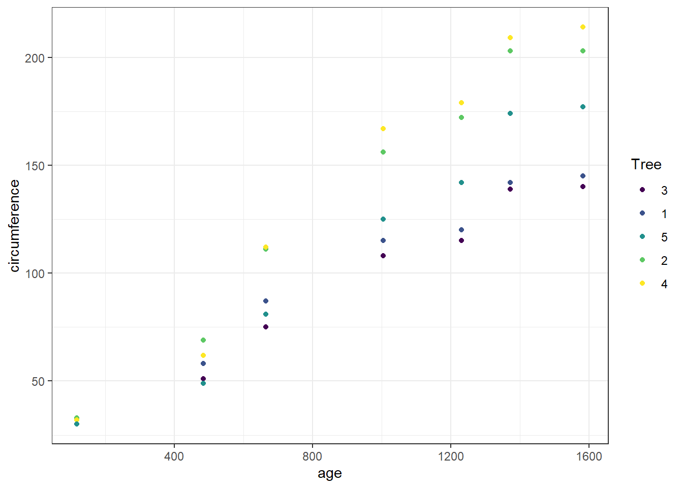
If its not working, run
blogdown::check_site() and follow the instructions next to the [todo] items.
4. load to github
In the files tab, navigate to the .gitignore file. Add so it contains the following .Rproj.user .Rhistory .RData .Ruserdata .DS_Store Thumbs.db /public/ /resources/
Now run
blogdown::check_gitignore()
#and
blogdown::check_content()Then commit the files and push to github.
Due to the massive number of files associated with the themes, we found it better to do the first commit through the shell
Tools>shell>git add -A
To authorise github, we found the best option to be to
Control Panel > User Account > Credential Manager > Windows Credential > Generic Credential
Then remove git credential
Then, when you push the repo it’ll ask you for credential through the browser.
5. Publish site!
Log into netlify (using github account). Then click new site from git, continuous deployment: Github. you should be able to see the repo from within netlify. Select deploy site.
It will give you a temporary URL which is live! Now it will automatically update every time you push changes to github.
To change the site name, general > site details > change site name
Now go back to R studio, and navigate to teh config (yaml or toml) and add in the correct url (probably around line 3)
Run Blogdown::check_netlify() to find any issues.
Part 2. publish vector data
Load necessary packages
library(sf)## Linking to GEOS 3.9.1, GDAL 3.2.1, PROJ 7.2.1; sf_use_s2() is TRUElibrary(tmap)Get the data
The process to get the data is stored in a script (scripts/get_osm_data.R), instead of integrating it into this R Markdown file. This allows us to not overload the data provider but always querying the API, every single time the article is rendered! (And we don’t need to process the data every time either.)
Here, we only need to read the data from a file that was previously created:
green_space <- st_read("data/green_spaces.geojson")## Reading layer `green_spaces' from data source
## `C:\Users\uqmrudg1\Desktop\blog_website\content\post\2021-10-28-creating-a-geospatial-blog-with-blogdown\data\green_spaces.geojson'
## using driver `GeoJSON'
## Simple feature collection with 5861 features and 3 fields
## Geometry type: POLYGON
## Dimension: XY
## Bounding box: xmin: 152.6764 ymin: -27.67486 xmax: 153.4664 ymax: -27.00613
## Geodetic CRS: WGS 84Visualise on a slippy map
The tmap package is useful to visualise vector data on a slippy map.
tmap_mode("view")## tmap mode set to interactive viewingtm_shape(green_space) +
tm_polygons(col = c("#43C467"), alpha = 0.5)Data is copyright OSM contributors but release under an ODBL licence.
Part 3. Publish Raster data
An example raster visualisation.
Load the packages
library(terra)## terra 1.5.17##
## Attaching package: 'terra'## The following object is masked from 'package:ggplot2':
##
## arrowImport the data
The data comes from the Bureau of Meteorology website, it is a raster file of average annual rainfall. We’ve put the file into a data directory, inside the blog post’s directory.
rain <- rast("data/rainan.txt")Inspect
rain## class : SpatRaster
## dimensions : 691, 886, 1 (nrow, ncol, nlyr)
## resolution : 0.05, 0.05 (x, y)
## extent : 111.975, 156.275, -44.525, -9.975 (xmin, xmax, ymin, ymax)
## coord. ref. : lon/lat WGS 84
## source : rainan.txt
## name : rainanOne single band, by default with the WGS 84 CRS.
The average rainfall for the whole raster is 451.61 mm.
Visualise
Make sure to add a caption to visualisations, and some alternative text if needed!
plot(rain)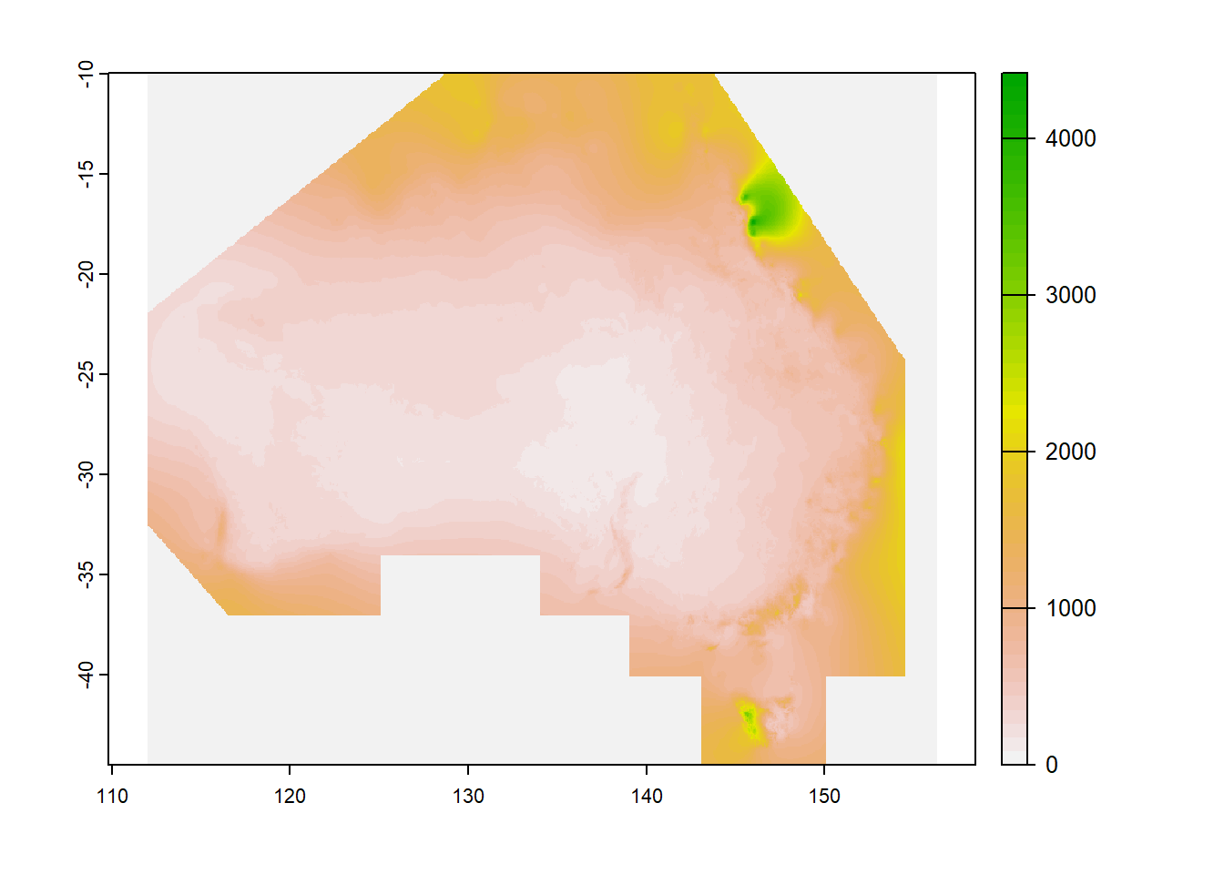
Figure 1: Average annual rainfall in mm (1980 to 2010)